Drilling technology: Autonomous drilling comes to life

Autonomy is an evolution—a journey from total human interface through automation and reduced human-machine interface to self-adjusting autonomy. The difficulty of the assignment is compounded by the challenges of subterranean drilling environments under instantly changing conditions. Only a concept in the minds of engineers not long ago, there is now realization of a self-steering BHA, capable of trajectory control without human intervention. The consequential benefits are holistic to the industry in terms of safety, sustainability, cost efficiency, accuracy, consistency and predictability. 

An autonomous BHA means fewer Directional Drillers (DD) are required on site, which exposes fewer personnel to HSE risks. Additionally, smaller crews mean less trips to rig sites, and combined with more consistent drilling performance, autonomy reduces both energy consumption and activity-related CO2 emissions while being more cost efficient. And because an autonomous BHA reacts instantaneously to changing downhole conditions—eliminating delays of data to surface to response—trajectory and well placement are more accurate. The pace toward autonomy increases with every field run. To date, more than 26,000 ft of curved section have been drilled autonomously on U.S. land, the Middle East and the North Sea. 

Challenge/solution. In the Permian basin, high shock and vibration, combined with high RPM while drilling along the north–south line, called the zone of exclusion (ZOE), made continuous while-drilling azimuth measurements difficult downhole. However, a BHA guided by autonomous technology drilled seven curves, on seven unconventional wells, on a particular asset, and compared it with offset wells on the same asset. The curves required 42% fewer downlinks, and the on-bottom drilling speed increased 39%. 

Another Permian basin operator built the curve and drilled the tangent—or the BHA did so, autonomously—resulting in no downlinks during the 579-ft curve, also increasing the rate of penetration (ROP) 39%. The BHA drilled all the way to the horizontal landing at 180° azimuth in the ZOE. A smoother trajectory was delivered on the 579-ft interval of curve with no downlinks. 

How is autonomous drilling being developed? The core philosophy behind autonomous trajectory control is a multi-layered primary-and-secondary-based approach in cascade, with which system complexity increases with additional layers. This methodology improves the overall trajectory-control-system efficiency when dealing with nonlinearities, delays and uncertainties present during drilling. This principle laid the groundwork for several operational modes of automated trajectory control for rotary steerable system (RSS) tools. 

Remaining and significant challenges facing trajectory automation were automated kick-off, automatic curve control for geometric and geological steering, and combining them into automated trajectory control by combining the surface and downhole information—representing higher levels of directional trajectory automation and control handled conventionally by the DD. This includes geometric and geological steering as an outer (primary) layer to the attitude controller. Autonomy removes these dependencies on surface intervention on downhole trajectory response, unlocking faster response to changing conditions when, and where, encountered downhole. 

Automated trajectory control. Two basic approaches for controlling a multivariate system like trajectory are either a multi-input and multi-output controller or a cascade-control approach that is a multi-layered primary-and-secondary-controller approach, with increasing control complexity achieved by adding additional layers to the control system. The cascade-control approach is better-suited for control applications, where a range of frequencies of interests must be addressed. In this configuration, the inner-loop control takes care of faster dynamics than are managed by the outer loops that are in the cascade. The cascade control is also useful in eliminating some of the disturbances and improving the dynamic performance of the closed loop. 

An open-loop trajectory propagation comprises input variables that are manipulated by the DD, such as weight on bit (WOB), RPM, flow and steering commands; the output of the process is the resultant trajectory. The BHA configuration and bit characteristics are considered constants during drilling. 

Fig. 1. Closed-loop trajectory control concept, using multi-input multioutput controller.

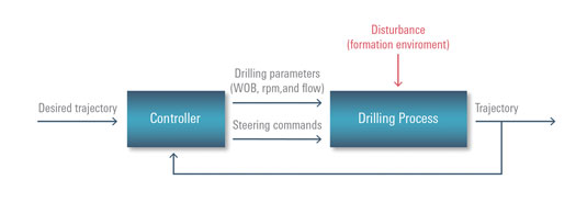
Then, there are the disturbances, such as the formation. These are added as input, because they influence resultant trajectory drilled. For the closed-loop trajectory control, the concept of the multi-input and multi-output case is shown in Fig. 1. The controller in this case uses desired trajectory as input and outputs the changes in the drilling parameters and steering commands to achieve the desired trajectory. Remember that the formation is a disturbance to the system. 

Fig. 2. Closed-loop trajectory control, using cascade control.

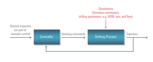
However, for the concept of the cascade control approach, besides the formation disturbance, the drilling parameters act as disturbances to the closed-loop system and any changes of the drilling parameters and formation are automatically corrected by the controller, Fig. 2. 

Automated trajectory control—cascade approach. After articulating the advantages of the cascade approach for trajectory control, the groundwork was laid for a generic approach to automating well placement using the cascade closed-loop approach with several layers of control (Ignova et al. 2014 and Matheus et al. 2012), Fig. 3. The formation represents the hole propagation measured, using accelerometers and magnetometers; it is affected by the steering and bias forces. The control/steering unit represents the first level of control; it computes the TF, based on sensor accelerometers and magnetometers, compares them with target TF and steering ratio (SR), and executes the steering force to modify the formation level. 

Fig. 3. Generic automation for well placement.

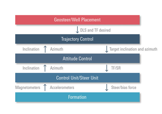
The attitude control represents the second level of control; it senses the continuous inclination and azimuth and computes the target TF and SR to be executed by the first level of control. Trajectory control represents the third level of control; using the target dogleg severity (DLS) and the desired TF direction, it computes the target inclination and azimuth to be executed by the second level of control. Geosteering/well placement represents the fourth level of control; it executes complex reservoir models to maximize well placement and specifies the target DLS to be executed by the third level of control. The telemetry rate between the RSS tools operated downhole and the surface plays a key role in making the design decision, where each control loop is going to be placed, either at the surface or downhole. 

Figure 3 illustrates attitude control already applied in cascade with the position control loop (Matheus et al. 2012). The attitude controller, besides playing the key role of maintaining the target angles, is also used to correct for the true vertical depth (TVD) error that could be due either to uncertainties in the geological model or TVD losses during the inner-loop disturbance control. 

Auto-curve curvature control. The curvature controller generates set-points for the inclination and azimuth targets, which are fed to the attitude controller, to produce desired curvature characteristics, automatically nudging those set-points. This auto-curve controller is an extension to the manual nudging of the attitude controller, Fig. 2. The auto-curve controller uses the information about the ROP to produce set-points for the inclination and azimuth fed to the attitude controller. ROP values are crucial, if the telemetry rate is such that the auto-curve controller operates downhole in the time domain. The ROP, itself, can be measured downhole, estimated, and controlled or downlinked to the tool. 

Auto-curve trajectory control virtual field testing. Virtual testing evaluates the performance of the control method and identifies and optimizes critical parameters of the controller (e.g., controller gains before actual field testing). Additionally, virtual field testing assesses limitations of the controller (e.g., sensitivity to disturbances such as ROP, WOB, and BHA configurations relevant to field location). 

Fig. 4. An advanced modeling system enables engineers to simulate trajectory automation and control by conducting a virtual field test to verify performance of the single auto-curve algorithm.

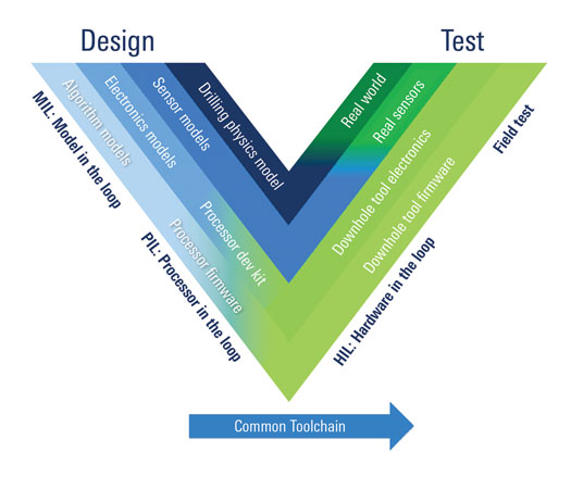
Testing control applications is traditionally done in a Simulink environment. If results are satisfactory, an appropriate specification and requirement document is sent to the software/firmware team, where the controller algorithms are coded and tested in hardware-in-the-loop-simulation (HILS) environment but without the feedback signal and plant model, which, in this case, is the hole-propagation model. This set-up does not perform real-time simulations for disturbances, such as formation changes, WOB, ROP and downlink/uplink delays. The closed-loop controllers are then evaluated in the field, which makes it expensive and limited in terms of how many parameter changes can be performed in one run. The environment is uncontrolled, and the number of sensors in the tools are limited; therefore, it is difficult to trace the causes of any failures. 

This traditional approach is well-suited for testing real-time answer products and estimation algorithms, but not for testing closed-loop trajectory control systems. A model-based digital design process was adopted and implemented to performance-test closed-loop trajectory controllers and accelerate from initial concepts to operations while identifying their risks and suitability early in the development process, minimizing failure risks. After satisfactory results were obtained with the design of the controller for the given requirements, the blocks of the control system were compiled and transferred to a real-time NI PXI system within the NI VeriStand environment. After the transfer to the real-time environment, the next stage in the design process was removing the individual components and replacing them with hardware blocks. 

The model-based control system development significantly boosted the maturity of the control system by testing control algorithms as a virtual system, well before they were implemented and integrated as software. The use of the plant- and controller-executable models made it possible to verify and validate the control systems for desired functional requirements in the initial stages of the design process. 

Virtual field test results. Trajectory automation and control were simulated by conducting a virtual field test (VFT) to verify performance of the single auto-curve algorithm, Fig. 4. These tests enabled identification of the effects of nonlinearities, delays and uncertainties that are present during drilling, further enabling identification and optimization of critical parameters for the controller. The system was tied to, and calibrated with, a real field example. 

The single auto-curve algorithm was run in three different modeling environments—initially Simulink, and then in an integrated drilling engineering analysis system, and in a model-in-the-loop simulation (MILS) for the VFT. The results from the same tests run in each platform were validated, matching up within a few feet of each other at total depth (TD). 

Conducted in two configurations, the first was a model-based test in the integrated dynamic engineering analysis system, drilling over 8,800 ft (19 runs). In this environment, the system was fully modeled, with the exception of the control unit. The goal of this test was to excite the system with drilling parameters and formation disturbances. All functions (except the control unit), ROP patterns, and perturbations, such as soft formations and formation push, were modeled. The second test was also mode-based but it used an MILS environment, in which over 24,400 ft were drilled (25 runs). In this environment, the entire downhole system was modeled; no hardware nor firmware was used. The downlink utilities were not in use; setpoints were linked to the models with a specific user interface. All functions were modeled; ROP patterns were predefined. 

To validate the testing environment, the simulations were tied into the well plan of a real field example in North America. This curve had a build of 8°/100 ft, and the DD used nine downlinks throughout the curve to land the well. The field example was not pure 2D, so a virtual 2D well plan was created from the Tie in Point (TIP) with the target coordinates as per the well plan. This enabled comparison of 2D results with a 2D well plan. The tests in the integrated dynamic engineering analysis system and the MILS generated similar results. 

For all these tests, the trajectories generated show what the curve looked like with no intervention or downlinking apart from the initial setting. TVD errors at TD were analyzed, as well as other KPIs. In reality, the DD or operator intervenes to adjust performance (if required) after a trend is established, so the error at TD is a hypothetical worst-case error and would only occur if nothing was done to correct trajectory. When the generated trajectory is closer to the well plan, the performance of the test is considered more successful. 

Initial tests used a constant ROP for the entire run. For each ROP tested, a constant drilling ROP is assumed as hole-propagation ROP and fed into the controller. Each test case consists of independent runs on the simulator, with selected ROP values as a reference and auto-curve ROP +/- percentage error as the test. The resultant trajectory was compared for sensitivity analysis. The auto-curve ROP input ranged from 30ft/hr to 450ft/hr, with most tests run with 200 ft/hr as the input to the hole propagation model. 

Initial ROP sensitivities were assessed, and results show that if the auto-curve algorithm has an ROP error of 20% higher than true ROP, the trajectory error generated [is similar to an 80% ROP error and] gives a TVD of approximately 100 ft too high at target TVD, and a larger displacement if the error is 20% lower than true ROP. Fine-tuned tests with smaller errors were performed (SPE-194727-MS), showing that overall ROP error throughout the well is critical but that fluctuation in ROP throughout the well is not. A key achievement was demonstrating the sensitivity of auto-curve input ROP to ROP variations in the hole propagation model. The resultant trajectory accuracy to the planned well path is a function of how accurate the ROP is, which is fed into the auto-curve controller. 

It is possible to calculate the ROP error (design an ROP observer at surface) and advise DLS nudges or corrections to ROP to make the TVD correction required during drilling. The TVD correction can be made by manually adjusting the DLS desired by downlinking a DLS nudge; alternatively, ROP can be adjusted by downlinking ROP or by controlled drilling or by automated downlinking of ROP in the future. 

The DD will make adjustments during drilling (as is done when running inclination hold or inclination and azimuth hold), and the auto-curve controller (even with a 10% error to ROP) would generate a predictable yield, which the DD would adjust to land the well in the correct place. There would be a smoother curve and fewer downlinks than the current manual method for drilling the curve. 

In addition, the DD or operator would not require as much skill or experience to make these adjustments and correct the well path. Although the DD deviated from the well plan and kicked off early, the turn was done early, and the trajectory converged to the target azimuth during the run, passing through the target within feet of the centerline. The MILS tests are pure 2D and follow a virtual 2D well plan, which is why they plot straight from the tie-in point to the target. They do not deviate from the well plan, and all end up within feet of the target in the virtual plan. 

The results of virtual field tests also helped evolve the single auto-curve algorithm into the current state of autonomy—the auto-curve mode behaves much like other automated modes, such as auto-inclination (inclination hold) and auto-tangent (azimuth hold), in that the DD engages the mode and tweaks the settings (DLS/TF/ROP) as required, depending on the trajectory generated. The auto-curve controller internally adjusts steering controls, such as steering ratio, and is real-world proven with results. But such proof points were made possible by the virtual field tests. These simulations enabled developing the workflows, algorithms, and data architecture needed for actual field trials, accelerating the evolution of autonomous BHAs. 

Path forward. Of course, fully autonomous BHAs are still ahead of us, but what’s being done today is evolving crucial capabilities such as auto-curve, which surmounts one of the last significant autonomy obstacles. And achieving this means dispensing with siloed, independent workflows that, in the long run, will reduce downlinks, increase drilling speed, improve drilling efficiency and minimize deviation from the plan with less tortuosity—all while helping to reduce associated emissions.  

*Mark of Schlumberger 

ACKNOWLEDGEMENT 

This article contains elements from SPE paper 194727-MS, which was presented at the at the SPE Middle East Oil and Gas Show and Conference, March 18-21, 2019. 

About the Authors

Maja Ignova

Schlumberger

Maja Ignova is a senior control engineer at Schlumberger. She has been with the company for more than 20 years. Her research interests and applications are in the field of automation and trajectory control for rotary steerable systems, drilling dynamics interpretation and machine learning. She holds a PhD in process modelling, optimization, and control from the University of Newcastle, UK.

Kate Mantle

Schlumberger

Kate Mantle is a directional drilling advisor for new product development at Schlumberger. She has been with the company for more than 30 years and has spent over 20 years working in the field. In 2017, she became directional drilling subject matter expert, working within the automation team at SHTC, UK. Her interests are currently trajectory control and automation. She holds a BSc Hons degree in geology from the University of Cardiff, Wales.