Big Data: What is a significant sample size?

What best distinguishes human beings from other animals is our foresight, so why do we get forecasting so wrong and so frequently, and don’t learn from our mistakes? For example, man is the only animal that trips twice over the same stone. We are used to saying that our portfolio will deliver a P90, P50, Mode, Mean or a success rate of X%, but that is only credible, or approaching credible, if the portfolio contains a statistically significant number of samples. One of the problems with our continuous surprise with failed predictions mostly derives from our lack of understanding of sample sizes.

A sample is a percentage of the total population in statistics. You can use the data from a sample to make inferences about a population as a whole. For example, the amount of variation of a set of values of a sample can be used to approximate the amount of variation of the population from which it is drawn. This is also known as the standard deviation. It is simply a measure of the amount of variation or dispersion of a set of values.

INFORMATION NOT DATA

Variance measures how far a set of numbers are spread out from their average value. Accuracy of prediction depends on the variance of the estimate. For averages of independent observations or prospect volume distributions, the variance goes down by 1/√n, where “n” is the sample size. So, in general for independent observations, the accuracy of an estimate improves as the sample size increases.

Fig. 1. Prospect volume distributions with same P50=250 MMbbl of oil but different variances.

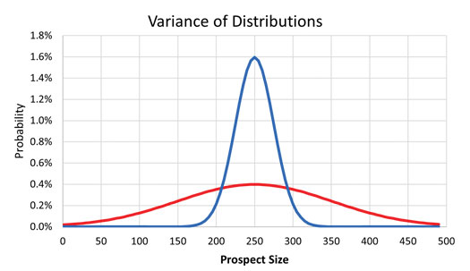
Figure 1 shows an example of prospects from two geological basins with the same P50/mean (250 MMbbl of oil) but different variances. The blue population has mean 250 MMbbl of oil and variance 625 (Standard Deviation=25), while the red population has mean 250 MMbbl of oil and variance 10,000 (Standard Deviation =100). NB: Variance is the average of the squared distances from each point to the mean, which is the mid-point (P50) for a normal distribution.

Statistical mathematics can be complex for many, so I will not go into any depth. But simply put, we can calculate the size of a significant sample of a population if we define what level of confidence we want in our prediction (e.g. low < 50%, high >90% etc.) and the size of the total population of data. We do not always know the exact size of the total population of data, but we can estimate this, and precision is not required.

We already have a problem with definitions by mixing everyday terms in public life with those of the oil and gas industry. For example, most oil and gas professionals associate “proven reserves” as having a 90% confidence level, yet the term “proven” in dictionary terms and in most legal cases is equivalent to over 99.99%. I shall, therefore, only refer to numerical confidence limits and try to avoid text-based descriptions like low, mid and high.

CONFIDENCE

Any forecast relies on two terms that you need to know. These are: confidence interval and confidence level.

1. The confidence interval (also called margin of error) is the plus-or-minus figure usually reported in newspaper or television opinion poll results. For example, if you use a confidence interval of 5, and 45% percent of your sample picks an answer, you can be reasonably assured that if you had asked the question of the entire relevant population somewhere between 40% (45-5) and 50% (45+5) would have picked that same answer.
2. The confidence level tells you how “sure” you can be. It is expressed as a percentage and represents how often the true percentage of the population who would pick an answer lies within the confidence interval. A 95% confidence level means you can be 95% certain; A 99% confidence level means you can be 99% certain.

When you put the confidence level and the confidence interval together, you can say that you are 95% sure that the true percentage of the population is between 40% and 50% in the example above. The wider the confidence interval you are willing to accept, the more certain you can be that the whole population answers would be within that range.

FACTORS THAT AFFECT CONFIDENCE INTERVALS

Three factors determine the size of the confidence interval for a given confidence level:

• Sample size
• Percentage
• Population size.

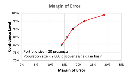
Confidence intervals are intrinsically connected to confidence levels. Confidence levels are expressed as a percentage (for example, a 90% confidence level). Should you repeat an experiment or survey with a 90% confidence level, we would expect that 90% of the time your results will match results you should get from a whole population. Simply put, the larger your sample size, the surer you can be that the answers from the sample truly reflect the whole population. This indicates that for a given confidence level, the larger your sample size, the smaller your confidence interval. However, the relationship is not linear (i.e., doubling the sample size does not halve the confidence interval)—Table 1 and Fig. 2.

Fig. 2. Margin of error for a portfolio of 20 prospects and a basin population of 2,000 discoveries and fields.

HUMAN BIAS IN SAMPLING

Sometimes the statistical conditions of using sampling are violated because of human bias or loose criteria in defining the population that the estimate is intended to cover. For example, the desired target population may be dry holes in a basin, yet when the estimate is made, certain sub-groups of wells are intentionally excluded (i.e. sample selection bias). This occurs, for example, if a geoscientist excludes such groups as missed pay or mechanically junked wells.

In contrast to probability sampling, there is no statistical theory to guide the use of non-probability judgmental sampling, which is a method that relies upon “experts” to choose the sample elements. As one would expect, this method of sampling varies from expert to expert and therefore yields different results each time. It’s one form of cognitive bias among many that are described by authors such as the seminal paper, “The difficulty of assessing uncertainty,” E. Capen.¹ Capen asked if there was some deep underlying reason that prevents us from doing better. The answer is “yes,” and it’s called heuristics and biases. All humans are subject to heuristics and biases, regardless of technical competency or level of education. This is the reason why “Calibration is King,”² and oil and gas projects should always be peer-reviewed.

THE GEOSCIENTISTS’ ENEMY

Many subsurface professionals look for short cuts, and in today’s Big Data work environment, many don’t question the results of their analyses. The biggest problem facing peer reviewers and geomodellers today is the “Belief in the law of small numbers.”³ Although the original findings were not based on geoscientists, the findings show that this belief is general human behaviour. I hope that most readers can find it within themselves to concede that geoscientists are human.

The study teases out the implications of a single mental error that people commonly make, even when those people in the study were trained statisticians. People mistook even a very small part of a thing for the whole (e.g.: all 14 gas fields in the East Irish Sea are associated with seismic anomalies, so all undrilled seismic anomalies in this basin must be associated with gas accumulations).

Even statisticians tend to leap to conclusions from inconclusively small amounts of evidence. They did this, even if they did not acknowledge the belief that any given sample of a large population was more representative of that population than it actually was. The smaller the sample size, the more likely it is unrepresentative of the wider population. The conclusion of the study was that people can be taught the correct rule, but they do not follow the correct rule when left to their own devices.

SAMPLE SIZE: A ROUGH GUIDE

The Central Limit Theorem essentially states that if you keep sampling a distribution, the distribution of the average/mean of your samples will approach a normal distribution, as the sample size increases, regardless of the shape of the whole population. So, the distribution of the sample averages will become a normal distribution, as sample size (n) increases and a general rule of thumb tells us that “n” needs to be ≥ 30.

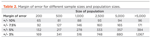
Before you can calculate a good sample size, you need some idea about the degree of precision you require, or the degree of uncertainty you are prepared to tolerate in your findings, Table 2. This table can only be used for basic surveys, to measure what proportion of a population of data have a particular characteristic (e.g. what proportion of fields use sand screens, what proportion of southern North Sea faults strike northwest to southeast etc.).

Maximum. While there are many sample-size calculators and statistical guides available, those who never did statistics at university (or have forgotten it all) may find them intimidating or difficult to use. A good maximum sample size is usually around 10% of the population, as long as this does not exceed 1000. For example, in a population of 5,000 North Sea wells, 10% would be 500. Even in a population of 200,000, sampling 1,000 mid-continent North American wells will normally give a fairly accurate result. Sampling more than 1,000 wells won’t add much to the accuracy regardless of how easy it is nowadays to process large data sets.

Minimum. Most statisticians agree that the minimum sample size to get any kind of meaningful result is 100 for household-type surveys, regardless of population size. If your population is less than 100, then you really need to survey all of them, or include qualifying statements about margin of error and confidence levels.

Sample size. Choose a number between the minimum and maximum, depending on the situation. Suppose that you want to assess the fracture stress of the Tertiary for mud weight calculations on the UK Continental Shelf, which has about 8,000 well penetrations. The minimum sample would be 100. This would give you a rough, but still useful, idea about the values. The maximum sample would be 800, which would give you a fairly accurate idea about the values.

Choose a number closer to the minimum if:

• You have limited time and money.
• You only need a rough estimate of the results.
• You don’t plan to divide the sample into different groups during the analysis (e.g.: Forties formation, Balmoral formation etc.), or you only plan to use a few large sub-groups (e.g. West of Shetlands, Central North Sea, Southern Gas basin).
• The decisions that will be made, based on the results, do not have significant consequences.

Choose a number closer to the maximum if:

• You have the time and money to do it.
• It is very important to get accurate results.
• You plan to divide the sample into many different groups during the analysis (e.g. different formations, depth of burial, etc.).
• You think the result is going to be wide-ranging.
• The decisions that will be made, based on the results, are important, expensive or have serious consequences.

ACCURACY

As well as the size of your sample and size of population, your accuracy also depends on the percentage of your sample that falls into your chosen categories. For example, if you’re unable to image Carboniferous faults in a field from a data room visit, you may want to, instead, rely on regional analogues. If 99% of your sample shows faults over 100 m throw strike northwest to southeast in the southern North Sea and 1% strike in a different orientation, the chances of error are remote, irrespective of sample size. However, if the percentages are 51% and 49% the chances of error are much greater. It is easier to be sure of extreme answers than of middle-of-the-road ones.

When determining the sample size needed for a given level of accuracy you must use the worst-case percentage (50%). You should also use this percentage, if you want to determine a general level of accuracy for a sample you already have. To determine the confidence interval for a specific answer your sample has given, you can use the percentage, picking that answer and get a smaller interval.

POPULATION SIZE

There are many situations when you may not know the exact population size. This is not a problem. The mathematics of probability prove that the size of the population is irrelevant unless the size of the sample exceeds a few percent of the total population you are examining. This means that a sample of 500 data points is equally as useful in examining the seismic velocity of 15,000,000 CDPs, as it would for a survey of 100,000 seismic CDPs. However, don’t forget about accuracy and confidence limits. Sometimes the detail in seismic velocity sampling does matter.

The confidence interval calculations assume you have a genuine random sample of the relevant population. If your sample is not truly random, you cannot rely on the intervals. Non-random samples usually result from some flaw or limitation in the sampling procedure. An example of such a flaw is to only analyze wells drilled by a specific operator. For most purposes, rate of penetration of drilling cannot be assumed to accurately represent the entire industry (majors and independents).

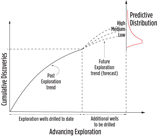
In mature basins, what we’re really forecasting with our analysis is the continuation of the basin creaming curve,⁴ with the assumption that the curve is not about to make a significant, or step change to its trajectory by drilling a relatively small number of new wells compared to the cumulative number drilled so far, Fig. 3. By plotting the new prospects on a probability density function containing all basin discoveries to date, it helps establish “reasonableness” that the new undrilled prospect is in line with discovery sizes, Fig. 4. In practice, this calibration approach falls apart in new plays, and frontier or sparsely drilled areas, where few data are available and following introduction of breakthrough new technology like 3D seismic.

Fig. 3. Creaming curve for calibrating predictions.

Fig. 4. Probability density function for field-sized distributions, East Irish Sea (P50 = 7.3 MMboe).

What we’re trying to achieve is to derive a set of figures that help us with our decision-making. A single number output from a “Black Box” type of analysis which is, at best, only partially understood by many decision-makers, is not what this author would describe as helpful. Decision-makers always want confidence of a return on investment, but what they really want to know is the likelihood that their capital budget will not be exceeded; what’s the likelihood that their reserves replacement ratio will stay above 100%; or what’s the likelihood that next year’s production targets will be achieved, if the chosen exploration program is drilled.

A single P50 value of X MMboe of exploration resources is only a single number, so we should be providing enough information to be informative, but not too much to overwhelm the end-user. Today’s probabilistic figures seem all too often to be quoted with an air of over-confidence, without the corresponding caveats and supporting qualifications.

CLOSING REMARKS

When oil and gas professionals look at investment portfolios, many are often misguided by natural bias, when they think they’re using seemingly robust statistical methods to make decisions. Hopefully, this article has highlighted the importance of sample size and an understanding of what confidence limits are.

A P50, for example, is the middle of a normal distribution, but the user is on shaky ground if the sample is small, compared to the population size, e.g.; forecasting the discovered resource outcome of a portfolio of 20 exploration prospects, drilled across five different geological basins, each with several hundred prior discoveries, producing fields and dry holes.

The reason being that the variance is going to be quite large, and there will, therefore, be a low degree of confidence in the mid-case (P50) value of the portfolio, in its use as a forecast for value of that portfolio. In these cases, it is recommended to use a Monte Carlo simulation, since the method uses the additional information contained in the entire prospect volume distribution (P99 through to P1) and is most beneficial to fully understand and appreciate the variance when the sample size is at its smallest.

By definition, for a normal distribution, P50 = Median = Mode (most likely). The descriptive term, “Most Likely,” is misleading, as it contains no information about variance. A confidence interval provides a useful index of variability, and it is precisely this variability that we tend to underestimate. The associated confidence is implicit in the P90/P50/P10 figures, but many upstream documents typically only report one of these (e.g.: P50) and therefore lose all information about variability. In the earlier example, of a resource distribution of a portfolio of 20 prospects, spread across five basins, it is advised to associate any reported single outcome with its associated confidence limit i.e.: P50 = X MMbbl of oil +/-20%.

REFERENCES

1. Capen. E, “The difficulty of assessing uncertainty,” Journal of Petroleum Technology, Vol. 28, Issue 8, 1976.
2. Ward, G., and S. Whitaker, “Common misconceptions in subsurface and surface risk analysis,” SPE paper 180134-MS, 2016.
3. Tverskey. A, and D. Kahneman, “Belief in the law of small numbers,” Psychological Bulletin, 1971, Vol. 76, No. 2, pp. 105-110.
4. Meisner. J, and F. Demirmen, “The Creaming Method: A Bayesian procedure to forecast future oil and gas discoveries in mature exploration provinces,” Journal of the Royal Statistical Society, Series A, Vol. 144, No. 1, 1981, pp. 1-31.

About the Authors

Gavin Ward

RISC Advisory

Gavin Ward has an economic, accounting and technical skill set from over 30 years in the oil and gas industry at major international operators and independents. He has peer-reviewed and valued assets and companies in Europe, Middle East, Far East, Africa and North America. Mr. Ward is an expert on risk and volume estimation, and is able to translate technical evaluations into meaningful economic and financial assessments as a chartered accountant/CPA and professional geoscientist. He has used these skills previously as a geophysicist for Phillips Petroleum; corporate business advisor for Noble Energy (based in Houston); Europe & Mediterranean portfolio manager for Noble Energy; Reserves and Economics manager for UK utility Centrica, and regional subsurface manager for Centrica Energy Upstream. He currently manages the EAME regional office, based in London, for RISC Advisory, a global technical energy consultancy. Mr Ward holds a B.Sc (Hons) degree in physics and geology from Aston University in the UK, an MBA from Cranfield School of Management in the UK, Dip M. Post Graduate Diploma in marketing, MCIM Chartered Institute of Marketing, UK; and is a fellow of the Association of Chartered Certified Accountants.