Artificial intelligence for automating seismic horizon selection
Artificial intelligence is being used in self-driving cars, vehicle identification, robotic vacuums, fingerprint identification and facial recognition. The next logical progression is to incorporate AI into seismic data interpretation. This article will provide evidence that automated seismic horizon selection is possible.
From a 2-column text file of time-amplitude pairs, an algorithm produces a reflection-time-ordered text file of all continuous series of connected pixel coordinates, easily read by mapping software. These connected pixels are plotted separately on the input seismic test line’s peaks and troughs. Over 10,000 connected segments were written in less than a minute of computer time, saving many hours of manual labor.
MOTIVATION
An inordinate amount of the time generating subsurface maps from seismic data is spent defining horizons by clicking a mouse on connected pixels, connected being the key word. Before this project was launched, I worked as an exploration geophysicist—with major and minor oil companies—for many years interpreting and processing seismic data, using some of the most advanced software for interpretation and processing.
I found that processing seismic data was much more intellectually challenging than seismic data interpretation, because dramatic improvements in image quality were possible with different processing parameters. Seismic data are extremely expensive to acquire. To offset the cost, companies expect their exploration teams to extract maximum value from the data—in terms of high-quality drilling prospects. Measurable improvements in numerical solutions to the wave equation, computer processing speed, computer network efficiency and lower computer costs have led to seismic images depicting the actual subsurface geology over the last 30 years. An effective seismic processing geophysicist is continuously challenged by new technology. The appearance of seismic interpretation software in the 1980s sped up the mapmaking process, compared to earlier, when maps were produced using sepias and drafting sets. But today, it is still a tedious process, using a mouse to connect the continuous pixels of a geologic horizon reflection.
Most oil companies require a candidate for employment to have a master’s degree in geoscience. Sadly, the possibly over-qualified new hire will spend exorbitant amounts of time—perhaps most of his/her career “connecting the dots” like a kindergartener would in a coloring book. Extensive internet research uncovered no evidence that horizon picking had been automated. There were apparently no web-published algorithms that seemed to have any relevance, but literature on facial recognition and fingerprint identification software gave me confidence that automating horizon selection is possible. That was my motivation for this project. At the time I started the project, identifying faces and matching fingerprints to people seemed far more complex tasks.1,2 Keys to the development of my horizon detection algorithm was an understanding of the meaning of seismic waveform connectivity and of how to sort the horizon data into depth-order.
Vast volumes of unused data. Oil exploration and geophysical service companies have millions of lines of seismic data that are partially interpreted, at best. What if a human connecting the dots became unnecessary? What if software could make the hundreds or thousands of often tedious and time-consuming decisions in advance for each seismic image by connecting the adjacent pixels? Then, those who interpret seismic data would have more time to truly interpret and to better understand the geologic and geophysical properties of the structures they have mapped.
More detailed and accurate mapping greatly enhances the understanding of subsurface geology and leads to more discovered reserves. More time spent on integrating the geophysical and geological properties into those maps also means fewer dry holes. The process will reduce the occurrence of blurry-eyed, mind-numbing tedium leading to poorly mapped drilling prospects.

Conventional mapping software. Current commercial geophysical mapping software, such as Petrel, 3DCanvas, and Kingdom, have a built-in facility to extend and propagate individual horizons picked with a mouse along the seismic section being analyzed and into the third dimension by following coded rules for adjacency. I have not found any previous examples where every horizon is picked and the truly complex part i.e., writing the coordinates of those detected horizons to a file in seismic time or depth order. Mapping software packages all have the facility to extend the horizon picked on a 2D image into the third dimension. A 3D surface can be formed by the software, but its “seed” needs to be manually determined.
At the beginning of the project, I was shown an example of detailed automated horizon-tracking but without any ordered text output. Finding peaks and troughs is a far much simpler task than finding them in depth-order. A simple for-loop will find every peak pixel, but only in top-to-bottom, side-to-side order.

INPUT DATA
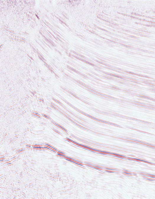
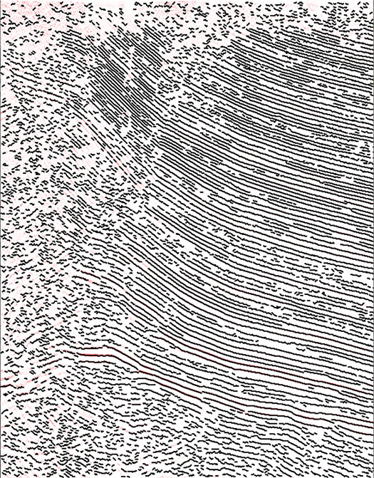
The proof-of-concept test data used here are a public domain vibroseis reflection-time section, of reasonable quality and from Rankin Springs, Australia, showing hydrocarbon-bearing potential—a possible 4-way closure with several fault traps, Fig. 1. Its image quality is middle-of-the-road (Goldilocks), which makes it ideal for proof-of-concept.
Worldwide, seismic data quality ranges from looking like a complete waste of money to showing such detail where you can “almost see” fluid movement within the horizons. If I chose the latter data type for the test case it might be said by some—will be said—that the data set made it easy, which is why I chose an older vintage, noisy but structurally interesting line. As it turned out, the algorithm is not prejudiced. This test line shows enough detail to understand the motivation for acquiring the data in the first place— possible fault traps and possible four-way closure—possible dome or plunging dome. There are patches of long, short and zero-continuity, clear fault terminations, conflicting dip and dead zones—dead zones in the most potentially hydrocarbon-rich, or at least most structurally complex part of the section.
The data were normalized after removing the overall mean from each trace. The brightest red signifies an amplitude of one. The brightest blue signifies an amplitude of -1. No color implies an amplitude close to zero. Tables of local minima, maxima and zeroes were computed from the normalized data and are the horizon detection code input.
RESULTS

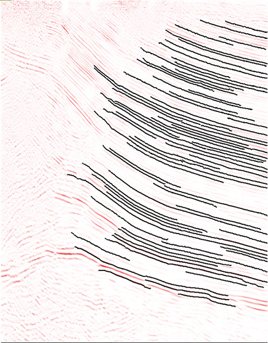
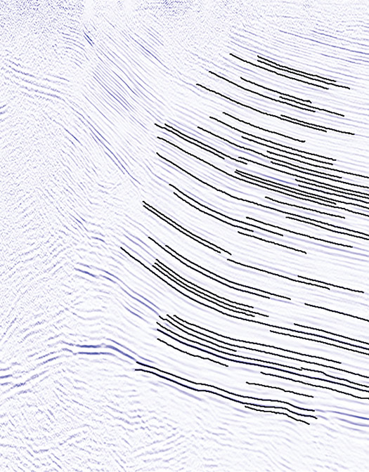
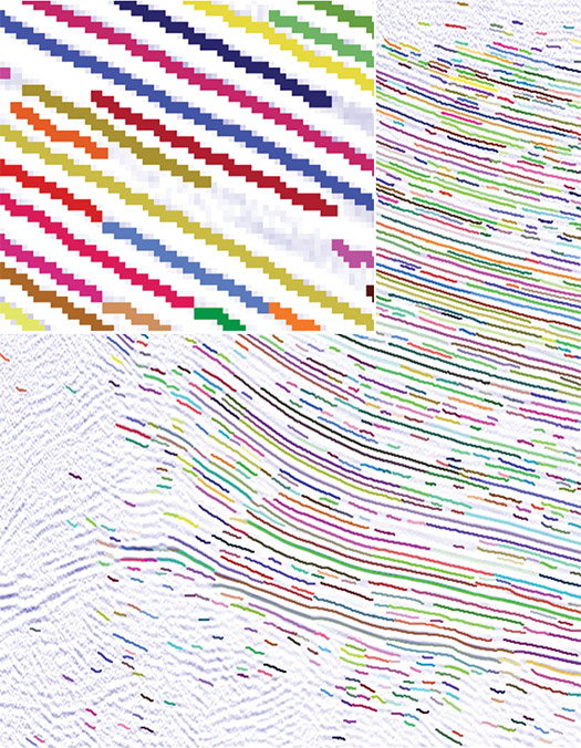
The images of horizons posted on the peaks and troughs of seismic amplitude sections verify proof-of-concept. Horizon lengths can be extended by conditioning the data with coherence filters, something I chose not to do, as I did not want the results to look artificial. However, for testing purposes a mild continuity filter was applied, and more horizons were captured. Compare Fig. 2 and Fig. 3. The remaining-pixels displays, Fig. 4 and Fig. 5, prove that every connection was found by the software, because every remaining peak pixel and every remaining trough pixel are isolated – surrounded by zeroes.

The results show perfect congruence of the detected peak and trough segments and the seismic data. There is no offset error. The code finds the absolute horizon position. It does not approximate horizon position. The discovered segments are congruent with the input local maxima and local minima. The output text files are in a convenient format, easily read by mapping software and humans—reflection time vs distance order (y-x pairs).
Code is extensible to 3D. All commercial 3D seismic interpretation software, as previously mentioned, have the facility to build surfaces connecting horizons at the same level in adjacent seismic lines along the z-axis or y-axis, as horizons are picked. If the test line here were part of a 3D survey, the output of the horizon detector code could be used as seeds to build 3D surfaces.
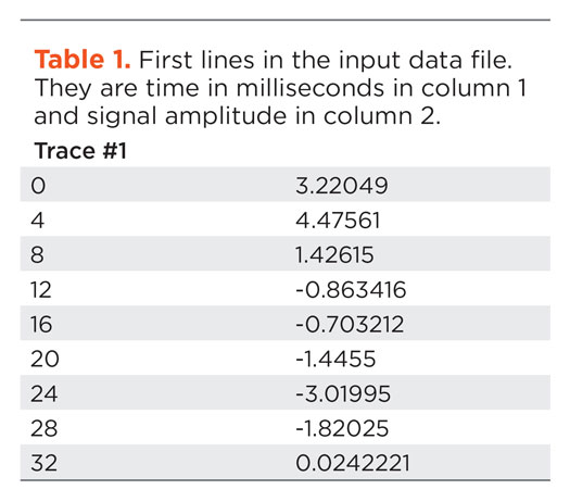
Details on input data. The input data is a two-column table of trace labels followed by times in milliseconds: 600 traces, 750 time samples, as it was found online as a public domain dataset, Table 1. Only one column would have been necessary, if the sample rate were published. It is a convenient format. No research was required to interpret a complex trace header. The type of amplitudes/signal is transparent to the code. Whether the amplitudes are time, depth, instantaneous frequency, phase, velocity—as long as there is visual continuity, my algorithm will track it.
This was the only data set used in the study. The amplitudes were used to compute and plot the relative amplitude seismic stacks, and the variation of amplitude is why the seismic sections vary in color intensity. After producing the seismic section plots, the above data were used to compute tables of local minima and local maxima. The local minima and maxima were written into tables, which were read by the horizon detection code, tables of trace number versus reflection time in negative ones for troughs and positive ones for peaks, Table 2.
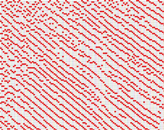
Both tables show small parts of the input data files: the first ten traces from 0 to 40 ms reflection time, Figs. 6a, 6b and 7. Another part of the input data set is shown within a spreadsheet in Fig. 8. It’s the part of the seismic section with the steepest geologic dip shown with red squares showing where the 1’s are. The ones represent local minima and maxima at particular reflection times but could represent one of many possible computed seismic attributes. The results would only have value, however, if there were linearity of the attribute within the seismic image.
Time saved by automation. The algorithm works extremely well in a minuscule fraction of the time it would take using commercial mapping software. On a core i-7 laptop, both the peaks and troughs segments, over 5,000 each, were picked in just under a minute. Preconditioning the data with an effective coherence filter will enable the algorithm to find many longer segments than it normally would on a noisy seismic section. All coding was in Java, which was chosen because of its great speed and its greater readability than C++.
If the subject seismic line were part of a 3D seismic survey in which all lines were the same length and as typical—there were both inlines and crosslines with the same number of traces as the test line here, say 600 inlines and 600 crosslines (1,200 seismic lines total)—that would require approximately 20 hr of computer processing time. On a distributed network of many nodes, the total processing time would be much less. On a small, distributed 20-node network, the processing time would be reduced to one hour. Assuming the input data here is a typical line and contains the average number of segments per line in this hypothetical 3D survey, then the number of horizons discovered would be 1,200 lines x 10,000+ peak and trough horizons for a horizon total of over 12 million.
A single geophysicist interpreting this hypothetical survey would spend months picking horizons—hopefully the key horizons—and end up with only a fraction of the horizons in the volume interpreted. The time saved by automation will allow geoscientists to be able to spend much more time incorporating geological and geophysical data into their seismic maps. These months saved by automation will dramatically help to speed up the decisions on whether and where to drill or not drill at a time when oil and gas inventories are painfully low.
REFERENCES
- Kellman, P.J., J. L. Mnookin, G. Erlikhman, P. Garrigan, T. Ghose, E. Mettler, D. Charlton and I.E. Dror, “Forensic comparison and matching of fingerprints: Using quantitative image measures for estimating error rates through understanding and predicting difficulty,” May 2, 2014 https://doi.org/10.1371/journal.pone.0094617.
- Zhou, H., A. Mian, L. Wei, D. Creighton, M. Hossny and S. Nahavandi, “Recent advances on single modal and multimodal face recognition: A survey,” IEEE Transactions on Human-Machine Systems, vol. 44, no. 6, pp. 701-716, December 2014, doi:10.1109/THMS.2014.2340578.
- Aramco's upstream digital transformation helps illuminate the path toward excellence (June 2024)
- Adopting a holistic approach to cybersecurity (March 2024)
- Embracing automation: Oil and gas operators leverage new operational efficiencies (May 2024)
- The five A’s on the road to completions automation (May 2024)
- Digital’s influence on drilling and production keeps growing (March 2024)
- Taming the red zone with automation (April 2024)